RNA-seq数据分析

RNA-seq hisat2 —— stringtie —— DESeq2 pipeline

1、需求

1.1 软件

linux安装：
hisat2 conda install hisat2
stringtie conda install stringtie
samtools conda install samtools=1.15.1
gffread conda install gffread

R包：
DESeq2 BiocManager::install('DESeq2')

1.2 数据

(1) fastq测序数据

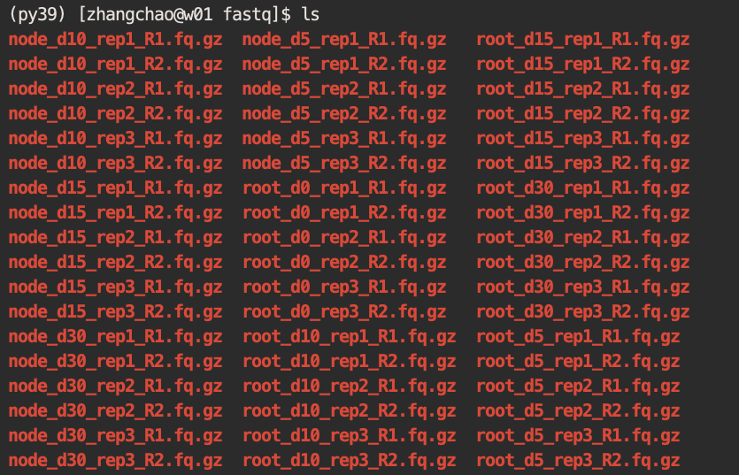
如图中例子，有9个样本，每个样本3个重复，双端测序

数据质控略

(2) 基因组及其gff注释文件，下载自Phytozome
gff转为gtf备用： gffread Wm82.gff3 -T -o Wm82.gtf

2、比对

2.1 构建索引

hisat2-build -p 8 path/to/genome.fa Wm82

2.2 准备config文件

ls path/to/fastq/*R1* > 1
ls path/to/fastq/*R2* > 2
ls path/to/fastq/*R2* | cut -d '/' -f 6 | cut -d '_' -f 1-3 > 0
paste 0 1 2 > align.config

2.3 比对

#!/bin/bash
hisat_index=/pub4/zhangchao/Methylome_Soybean/Reference/index/Wm82
cat align.config | while read id;
do
arr=($id)
fq2=${arr[2]}
fq1=${arr[1]}
sample=${arr[0]}
hisat2 -p 20 -x ${hisat_index} -1 $fq1 -2 $fq2 -S ${sample}.sam 2>${sample}_hisat.log
grep "NH:i:1" ${sample}.sam > ${sample}_unique.sam      #仅保留唯一比对
samtools view -H ${sample}.sam > ${sample}_head.sam
cat ${sample}_unique.sam >> ${sample}_head.sam
samtools sort -@ 20 -o ${sample}.bam ${sample}_head.sam
samtools index ${sample}.bam
rm ${sample}_unique.sam
rm ${sample}_head.sam
stringtie -p 20 -G path/to/Wm82.gtf -e -B -o ${sample}.gtf -A ${sample}.tsv ${sample}.bam
done

2.4 从tsv文件提取fpkm信息

ls *tsv|cut -d '.' -f 1|while read id;
do
nohup cat ${id}.tsv | awk -F "\t" '{print $1"\t"$8}' > fpkm/${id}.fpkm &
done

2.5 从gtf文件提取count信息

ls path/to/gtf/*gtf > gtf
ls path/to/fastq/*R2* | cut -d '/' -f 7 | cut -d '_' -f 1-3 > name
paste name gtf > prepDE.list
python path/to/prepDE.py -i path/to/prepDE.list -g prepDE_counts.csv -t prepDE_transcript.csv
sed 's/,/\t/' prepDE_counts.csv > all_count.txt

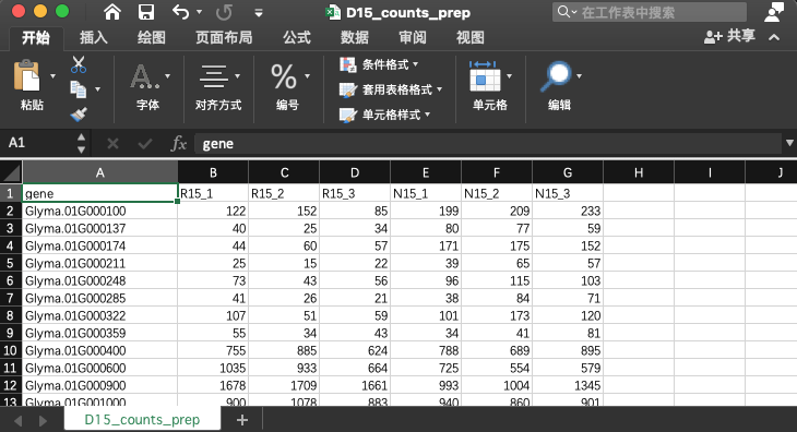
3、差异基因分析

DESeq2以基因count为输入文件

以15天的大豆根和根瘤为例：

3.1 DESeq2差异分析

将基因count文件下载到本地，使用R包DESeq2进行差异分析

rm(list=ls())
options(stringsAsFactors = F)
library(DESeq2)
library(tidyverse)

counts <- read_csv('path/to/D15_counts_prep.csv')
exprSet <- counts[,2:7]
rownames(exprSet) <- counts$gene

group_list <- factor(c('R15','R15','R15','N15','N15','N15'),
                     levels=c('R15','N15'))
colData <- data.frame(row.names=colnames(exprSet),
                      group_list=group_list)

dds <- DESeqDataSetFromMatrix(countData = exprSet,
                              colData = colData,
                              design = ~ group_list)
dds <- DESeq(dds)
sizeFactors(dds)
res <- results(dds)
res_d <- subset(res,abs(log2FoldChange) > 1 & padj < 0.05)

DEG <- as.data.frame(res_d)
DEG <- na.omit(DEG)

D15_up <- DEG %>%
  filter(log2FoldChange>0)
D15_up <- tibble(rownames(D15_up))
names(D15_up) <- c("ID")
write_tsv(D15up, file='D15_up.txt')

D15_down <- DEG %>%
  filter(log2FoldChange<0)
D15_down <- tibble(rownames(D15_down))
names(D15_down) <- c("ID")
write_tsv(D15down, file='D15_down.txt')

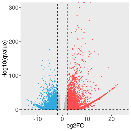
#火山图
threshold <- as.factor(ifelse(DEG$padj < 0.05 & abs(DEG$log2FoldChange) >= 2,
                      ifelse(DEG$log2FoldChange >= 2 ,'Up','Down'),'Not'))
ggplot(DEG,aes(x=log2FoldChange,y=-log10(padj),colour=threshold))+
  geom_point(size=0.5,alpha=1)+
  labs(x='log2FC',y='-log10(qvalue)')+
  ylim(0,300) + xlim(-15,25)+
  scale_color_manual(values=c("#30A9DE",'grey',"#ff4e50"))+
  geom_vline(xintercept = c(-2, 2), lty = 2,colour="#000000")+
  geom_hline(yintercept = c(1), lty = 2,colour="#000000")+
  theme(panel.grid = element_blank(),
        axis.text=element_text(size=14),
        axis.title=element_text(size=14),
        legend.position = "none"
        )